When are Rift Models relevant for the Petroleum System ?

There are currently contrasting views on the way strain is distributed within the lithosphere during rifting and the formation of passive continental margins, with direct implications for the subsidence and heat flow histories of the overlying sedimentary basins, and potentially also for the timing and degree of source rock maturity in these systems.

According to some authors, the asymmetry observed between most conjugate margin pairs (e.g. West Iberia-Newfoundland, East Coast USA-NW Africa, NE Brazil-West Africa and the Southern Australia-Antarctica) results from the activity of low-angle normal faults (detachments), which shift the region of pervasive upper crustal thinning and normal faulting (lower plate) from that of intense lower crust and mantle lithosphere thinning (upper plate; see Rosenbaum et al., 2008 and references therein). A paradoxical observation, nevertheless, is that in most margins the extension measured from normal fault throws appears to be much smaller than that inferred from subsidence and gravity modelling, thus implying ubiquitous upper-plate rift margin settings (the “Upper Plate Paradox”; Driscoll & Karner, 1998; Davis & Kusznir, 2004). 

Pervasive depth-dependent stretching (DDS) is also implied in dynamic models of rifting to explain features such as the deposition of salt over extremely thinned crust (e.g. off western Angola) and the exhumation of continental mantle prior to breakup in magma-poor margins (e.g. the West Iberia Margin; Lavier & Manatschal, 2006; Huismans & Beaumont, 2011). In contrast, results from a recently published kinematic rift model suggest that the crustal structure and subsidence along most passive continental margins can be explained assuming an essentially depth-uniform strain distribution through time (Crosby et al., 2011). Alternative models have also been put forward to explain the apparent deficit of extension in the brittle upper crust, namely by Reston (2005) and Ranero & Perez-Gussinyé (2010), who argue that the amount of extension accommodated in normal faults may have been largely underestimated in earlier studies.

The figures below illustrate the results from two simple experiments in actively explored rift settings: (Figure 1) the North Sea; and (Figure 2) the Angola passive continental margin. The pseudo wells were built from published seismic data and assume a simplified stratigraphy, where the thin black layers correspond to the location of two hypothetical source rocks in each setting. For simplicity all models assume a constant temperature at the base lithosphere of 1330⁰C, and the source rocks use a Type II, marine shale kerogen facies, with an initial TOC of 5% wt and HI of 500 mg/g TOC. The impact of varying the rift model assumptions is then evaluated in terms of the SR’s maturity.

 

The North Sea comprises a series of rift basins that formed over a sequence of extensional pulses between the Permian-Triassic and Early Cretaceous, interspersed with periods of thermal quiescence, volcanic activity and doming (Ziegler and Cloetingh, 2003). The Pseudo-well in this experiment was built from a NW-SE seismic constrained transect redrawn from Bell et al. (2014), at a location where the inferred total stretching factor (β) is 2; i.e. the crust, or the whole lithosphere, have been stretched to half their initial thickness during rifting (if the rift is assumed instantaneous; McKenzie, 1978). For the purposes of the experiment it is assumed that all extensional deformation took place during the Late Jurassic (160-150 Ma), except in the last scenario, where most thinning occurs during an earlier rift stage, in the Permian (260-250 Ma), in agreement with the published profile (see Bell et al., 2014 and references therein). 

The models show that changing the amount of lithosphere thinning within a reasonable range (black lines), imposing significant differential stretching between crust and mantle, has some impact on the timing/degree of maturity of the deeper, pre-rift SR. This results from differences in the post-rift thermal structure of the basin combined with rapid sediment burial. However, a similar effect is obtained by varying the steady state thickness of the lithosphere by only ±10 km, often beyond realistic model constraints, and a greater impact is even predicted when distributing the extensional deformation over several rift events (or varying the duration of rifting). The maturity of the shallower SR is independent of the rift model, although some differences are noticed for variations in the thickness of the steady state lithosphere.

 

The Angola (deep) passive continental margin formed due to intense stretching during the Early Cretaceous (mostly Berriasian-Aptian) followed by a transition period of thick salt deposition (Aptian) and continental break-up (e.g. Teisserenc & Villemin 1990). The transect shown above is redrawn from Lentini et al. (2010), based on deep seismic reflection and refraction data. At the location of the Pseudo-well the present day thickness of the crust is 8 km, measured between the base of the sediments and the Moho. For the experiment it is assumed that all extensional deformation took place during the Early Cretaceous (145-135 Ma) and that the initial crustal thickness is 32 km (i.e. β_crust = 4).

In the margins, where the lithosphere stretches to infinity prior to break-up, depth dependent stretching (DDS) may have a greater impact on the distribution of heat during and following rifting, and thus in the maturity of SR’s. In the experiment above this is observed when varying the amount of stretching in the mantle (β_mantle) between a factor of 3 and 4. For higher stretching factors, in this particular setting, the increase in heat flow converges asymptotically. The models also show, however, that similar magnitude effects, or even more pronounced, are produced when varying the thickness of the lithosphere and/or the duration of the rifting events. As in the case of the North Sea experiment the maturity of the shallower SR is independent of the rift model.

In summary, the experiments discussed here show that the implications of assuming conceptually different rift models for the timing and degree of source rock maturity in these settings may be of the same order of magnitude, and thus indistinguishable, from those inherent to the uncertainty in the parameterization of the rift model, such as the thickness of the underlying lithosphere and the age and duration of the rift events. Moreover, it is likely that the maturity of most syn- and post-rift source rocks does not depend significantly on the rift model, but mostly on the rate of post-rift burial. As good practice, these effects should be tested in order to identify the key sensitivities of the basin model, at least within a first order approximation.

 

References:

Bell, R. E., C. A.-L. Jackson, P. S. Whipp, and B. Clements (2014), Strain migration during multiphase extension: Observations from the northern North Sea, Tectonics, 33, doi:10.1002/2014TC003551.

Crosby, A. G.,  N. J. White, G. R. H. Edwards, M. Thompson, R. Corfield, and L. Mackay (2011). Evolution of deep‐water rifted margins: Testing depth‐dependent extensional models, Tectonics, 30, doi:10.1029/2010TC002687.

Davis, M., and N. Kusznir (2004), Depth-dependent lithospheric stretching at rifted margins, in Karner, G. D., Taylor, B., Driscol, N. W., & Kohlstedt, D. L (eds), Rheology and Deformation of the Lithosphere at Continental Margins, pp 92-137 Columbia University Press.

Driscoll, N. W., and G.D. Karner (1998), Lower crustal extension across the Northern Carnarvon Basin, Autralia: Evidence for an eastward dipping detachment, Journal of Geophysical Research, 103, 4975-4992.

Huismans, R., and C. Beaumont (2011), Depth-dependent extension, two-stage breakup and cratonic underplating at rifted margins, Nature, doi:10.1038/nature09988.

Lavier, L.L., and  Manatschal, G. (2006) A mechanism to thin the continental lithosphere at magma-poor margins, Nature, 440, doi:10.1038/nature04608.

Lentini, M.R., S. I. Fraser, H. S. Sumner and R. J. Davies (2010), Geodynamics of the central South Atlantic conjugate margins: implications for hydrocarbon potential, Petroleum Geoscience, 16, 217-229, DOI 10.1144/1354-079309-909.

McKenzie, D (1978), Some remarks on the development of sedimentary basins. Earth and Planetary Science Letters, 40, 25-32.

Ranero, C.R. and M. Perez-Gussinyé (2010), Sequential faulting explains the asymmetry and extension discrepancy of conjugate margins, Nature, doi:10.1038/nature09520.

Reston, T.J. (2005), Polyphase faulting during the development of the west Galicia rifted margin, Earth Planetary Science Letters, 237, 561-576, doi:10.1016/j.epsl.2005.06.019.

Rosenbaum, G., R. F. Weinberg and K. Regenauer-Lieb (2008), The geodynamics of lithospheric extension, Tectonophysics, 458, 1-8.

Teisserenc, P. and J. Villemin (1990), Sedimentary basin of Gabon; geology and oil systems, in Divergent/passive Margin Basins, AAPG Memoir 48, 117–199.

Ziegler P. A. and S. Cloetingh (2003), Dynamic processes controlling evolution of rifted basins, Earth-Science Reviews , 1-50, doi:10.1016/S0012-8252(03)00041-2.

 

Measuring the "maturity" of a hydrocarbon fluid

Geochemical analysis of a gas, condensate or oil can provide a lot of useful information about its origin. In the best cases this can include the type of organic matter in the source rock, whether it is clastic or carbonate, the depositional environment (terrigenous, lacustrine, marine, evaporitic) and whether it is has been altered by secondary processes (e.g. phase separation, biodegradation). In some cases, the presence of absence of certain marker compounds (e.g. oleananes, 24-isopropyl cholestanes) places broad limits on the age of the source rock.

Many geochemical reports also speak about the "thermal maturity" of a fluid. It is not always clear what is meant by this term but generally it seems to mean the maturity of the source rock from which the fluid was expelled. There are several kinds of geochemical maturity indicators, but most are either based on systematic relationships among gas isotopes (carbon or hydrogen), on ratios formed from isomeric compound pairs having differing thermal stability (e.g. sterane or methyl phenanthrene isomers) or on the concentration of thermally resistant compounds such as the diamondoids. Fluids with more of the thermally stable species or isomers are considered to have been expelled from a source rock at a more advanced stage of kerogen conversion.

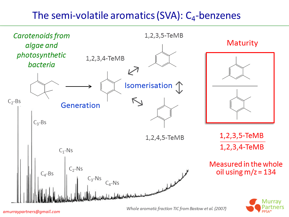
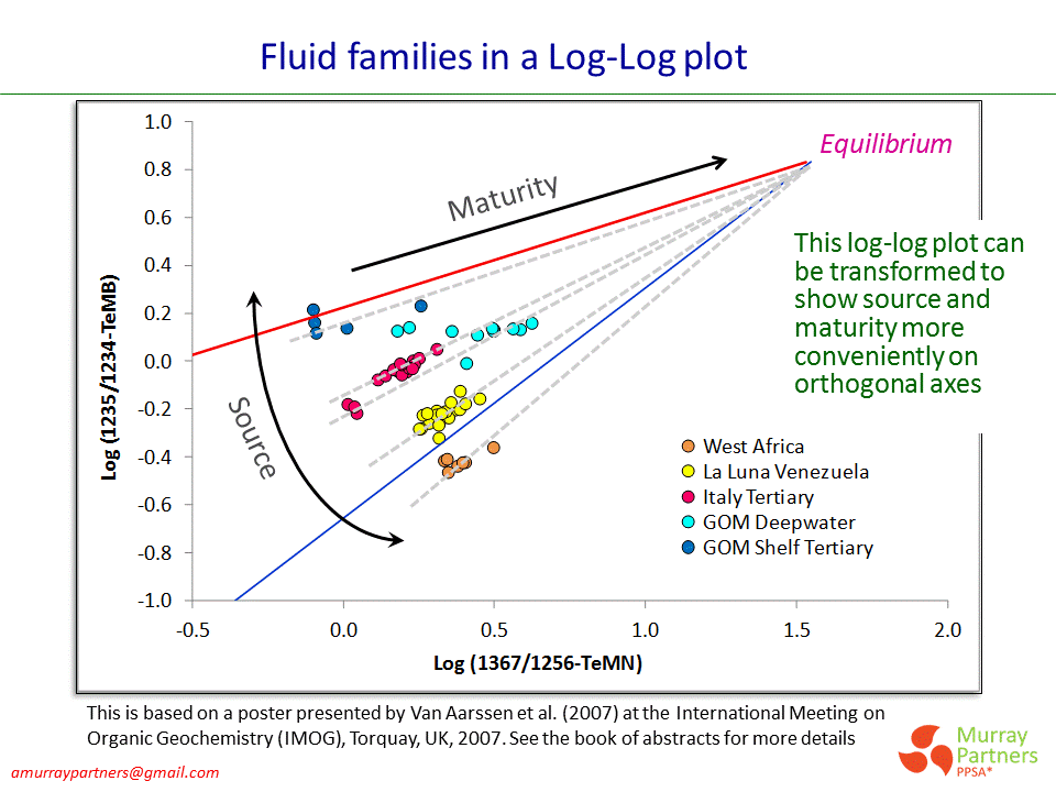
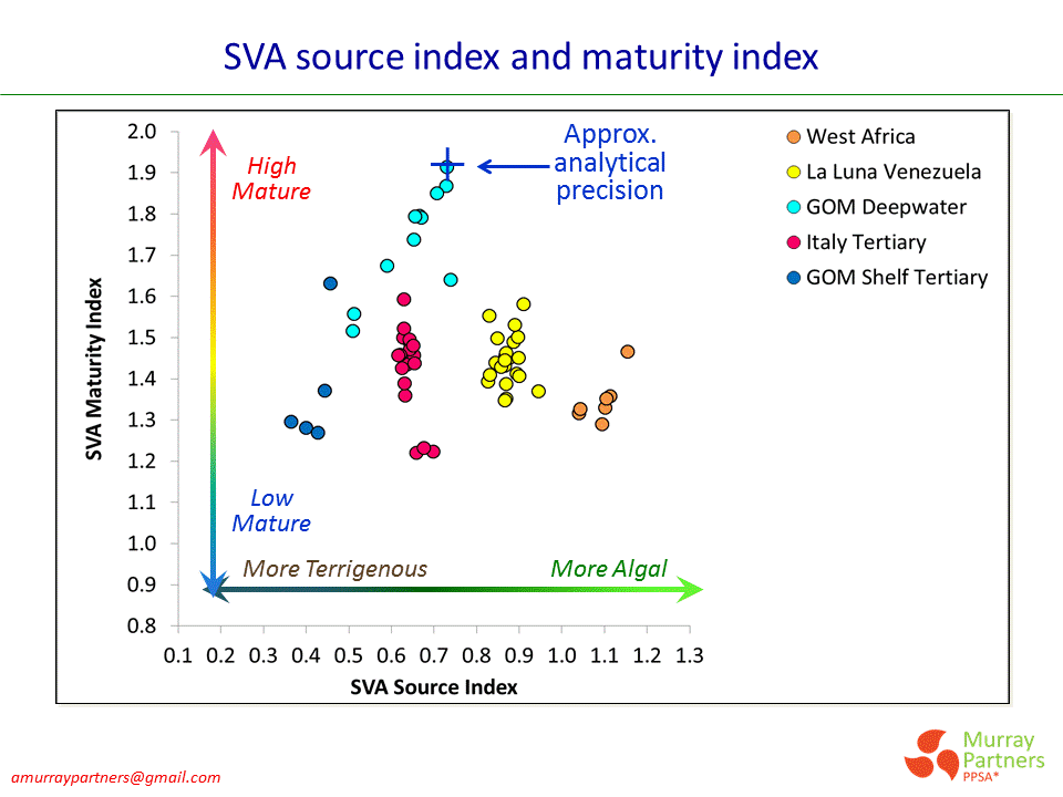
There are several fundamental problems with the concept as described above - but that is a topic for another day. For now, I would like to describe just one method of saying something about the "maturity" of a fluid sample. This is a method based on the relative abundance of two tetramethyl benzenes and two tetramethyl naphthalenes. These are mono- and fused diaromatic compounds containing 10 and 14 carbon atoms respectively. These compounds have boiling ranges straddling the range where we most commonly see a change from a gas-condensate fluid to a volatile oil. For convenience we call them the "semi-volatile aromatics" or "SVA". The method has been in use in a few companies for several years but has never been published, except in the form of a poster presented by Ben Van Aarssen at the International Meeting on Organic Geochemistry (IMOG) in 2007. A description of the method can be found in the book of abstracts for that conference. At that time, the SVA "maturity index" had not been calibrated to an equivalent vitrinite reflectance for the expelling source rock. There is also an SVA source index - derived from the same compounds and analysis - which gives an indication of degree of "algal" vs. "terrigenous" organic matter contribution to the source rock.

Some aspects of the SVA method are described below. I hope to get the time to write it up properly over the next year (in conjunction with Ben Van Aarssen). The bottom line is that it gives (we believe) a more robust indication of relative fluid maturity than most other methods. This arises from (a) a clear separation of the source and maturity effects (b) a basis in compounds which are present in reasonably high concentration in both gas condensates and oils and (c) a response range that extends from the earliest onset of fluid expulsion to well beyond the point at which gas becomes the dominant product. Calibration to absolute source rock maturity is more problematic - and may not even have a simple physical meaning,  as described in the last few few figures. This is an issue of particular relevance to shale oil/gas plays where - as per the previous blog entry - we often want to know how much of the fluid we produce was generated locally as opposed to being migrated in from more mature section elsewhere.

Happy Modeling :)

How fast can oil and gas migrate in the Eagle Ford shale ?

In view of increasing evidence for migration in some of the shale plays (since it has become common practice, should we still call it unconventional?), I wanted to try to  estimate the migration rates in the shales, using he Eagle Ford as an example.

Darcy's law states that at 1 Darcy (D) permeability, a fluid with 1 centipoise (cP) viscosity will flow 1 centimeter per second under a pressure gradient of 1 atmosphere (14.7 psi) per centimeter. That translates to about a rate of 0.000073 ft/sec at a gradient of 1 psi/ft.

At typical reservoir conditions, gas viscosity is around 0.01 cP, and the permeability of the shales are known to range between 1 nano darcy (nD) to 10 micro darcies (μD) or more. At hydrostatic conditions, the buoyancy gradient for typical gas (static water gradient is 0.43 psi/ft  and 0.13 psi/ft for gas) is 0.3 psi/ft. There are about 3.16 x10 ¹³ seconds in a million years. The Eagle Ford dips at about 30 meters per kilometer, meaning the lateral buoyancy gradient is about 0.009 psi/ft. Given all these, gas migration rate up dip along a 1 μD permeability zone would be

Migration rates (ft/my) = (0.000073*0.009) (psi/ft) x 10^-6 D x 3.16x10¹³ (sec/my) /  0.01 cP = 2082 ft/my (635 m/my) **.

The gas window part of the Eagle ford is quite over pressured, and the pressure gradient may be around 5000 psi over 50 km (=0.1 psi/ft, or about 10 times higher than the buoyancy gradient) which can result in 10 times the above migration rate. Higher rates would be possible in zones if the permeability is 10 μD or higher. The Eagle ford has been generating gas for more than 10 million years so this could add up to fairly long distance migration. Imagine what would happen in the Permian basin where the source rock was mature since 200 million years ago.

Since the incline (dip) is (30 m/km) and the permeability anisotropy (kx/kv) is is at least 100 to 1000 times, the process still favors lateral migration rates by 3 to 30 times. Perhaps lateral migration in the shales is more common than we have thought?

This could also partly explain some of the higher than expected GORs we see at relatively low maturity. Some of the gas condensates may have migrated up dip to mix with the oil. Since oil viscosity is 100 times that of gas, and a one third in buoyancy gradient - so it would migrate 300 times slower. The vast difference in migration rates in the oil window and the gas window creates a super sized natural dynamic trap. The difference in over pressure gradients may also provide additional help in this regard.

** note an earlier version of this post had a mistake in conversion that resulted in much higher rates. Thanks to Andrew for finding the mistake! 

The Signal and the Noise

Some time ago Zhiyong pointed me to Nate Silver's book "The Signal and the Noise" which is about the science of prediction. I'm now reading it again and in fact go back to it regularly because it is, I believe, essential (and sobering) reading for anyone engaged in the modeling business.

One of the key things I took away from this book is the human tendency to psychologically "anchor" on any scenario which we have put a lot of time and effort into constructing. This is a real danger for anyone who has toiled through the process of building a 3D model for a basin where much data gathering, entry, mulling over input parameters, resolving IT issues etc is often necessary to reach the point where the model can be executed. This typically takes days to weeks in my experience. Then, depending on the size of the model, it might take hours to days to complete a single run. At the end of this process one is well and truly "anchored" on the particular scenario chosen in the process of setting the model up. It is very hard, and very time consuming, to then go back and test alternative scenarios. It has been made easier by recent software and hardware improvements but it is still a difficult thing to do psychologically.

In training courses I am fond of a particular analogy for the model building process which involves some pictures of bridges. The idea is that any model is a framework of physical law that we use to connect the known (data, analogs etc) to the unknown (our target play or prospect). We need both good data and a good framework to build a good bridge and so get to the other side safely. In a way, the model algorithms encode prior knowledge (in the Bayesian sense) about how petroleum systems work in general, hopefully preventing us over-fitting our data and indulging in the wilder of our fantasies.

While reading the book last week an old and favourite movie appeared late one night on the TV. This was David Lean's classic 'The Bridge on the River Kwai", Alec Guinness in the lead role. For those who don't know this movie, the story describes a group of English prisoners in WWII Thailand, being forced by the Japanese to build a rail bridge over the river Kwai. The martinet colonel (Guinness) keeps his soldiers alive, in the face of appalling mistreatment, by giving them the focus of building the bridge. At the end of the movie the bridge is complete and the first Japanese train about to cross it. The British plan, all along, was to blow up the bridge with hidden charges just as the train crosses. However, when it comes down to it Guinness cannot bring himself to blow the bridge and tries to prevent it. He has become "anchored" to the bridge through the pain and toil of building it and is unable to see the "bigger picture" of hampering the Japanese war effort.

Happy Modeling

Using fluid inclusions to infer the presence of a paleo hydrocarbon column

Analysis of diagenetic fluid inclusions, whether by optical or chemical means, is a technique used to learn something about a petroleum system. The main utility is for old wells where no fluids samples are available and where all that remains may be some old cuttings in a store.

One of the best known methods is "fluid inclusion stratigraphy (FIS)" provided by Fluid Inclusion Technologies (FIT) in Tulsa, USA. FIS is one of many possible fluid inclusion analysis methods which can perhaps be grouped together under the term "Microshows".

A common question asked of fluid inclusion data is "Was there ever a hydrocarbon accumulation in my (now water wet) reservoir ?" In other words, is there a paleocolumn ?" The government research body in Australia (CSIRO) uses the "grains with oil inclusions (GOI)" method which involves counting the number of grains with oil inclusions visible through a microscope under UV light and expressing the result as a percentage (%GOI). CSIRO suggests a threshold of 3.5% GOI as the minimum consistent with a paleocolumn. From calibration studies in one province my company set a similar threshold for the FIS paraffin response some years ago.

Any comparison between optical and chemical indicators of fluid inclusion "strength" is difficult. For both practical and theoretical reasons we would not expect a simple relationship between the two. For one thing, an optical method such as %GOI counts the frequency of grains with visible oil inclusions whereas FIS measures the concentration of volatile hydrocarbons (and other species) released by crushing a bulk sample. Obviously, if the sample has a few big inclusions it would give a smaller GOI and larger FIS signal cf. one with a lot of small inclusions. There are several other reasons why the measures are not equivalent. However, we would at least hope that they would give the same answer to the question of paleocolumn presence or absence.

The figure below shows the results of a comparison for 49 samples from 9 wells. In all cases, where GOI indicated a paleocolumn FIS agreed. Similarly in most cases where GOI indicated no paleocolumn, FIS agreed. However, there were a few samples where FIS indicated a paleocolumn and GOI did not. From the location of these samples (all from one well) and the signal character it is likely that this is a paleo-gas condensate zone and hence the optically detectable oil inclusions are rare. This comparison is for one particular province and I cannot warrant that it would work out this way for other geological circumstances. 

So what does all this mean for evaluation of a petroleum system ? Clearly if we found that the target reservoirs in dry holes had high fluid inclusion abundance we might conclude that trap breach rather than lack of charge was the reason for failure. If the abundance is high enough we could carry out further analysis to permit oil-source or gas-source correlation to confirm activity of the prognosed source rock or the presence of a previously unrecognised one. We would hope to be able to do this on simple extracts of the cuttings (rather than on the tiny amounts in fluid inclusions)  but this isn't always feasible due to loss during storage or severe contamination with drilling mud. 

How to Calculate "Organic Porosity" for a Shale?

Here is a simple formula for calculating "organic porosity" formed as a result of converting kerogen to petroleum. 

Organic porosity (% rock volume) = TR(fraction)*HI (mg/gTOC)*TOC(% weight)*2.5/1.2/1150,

where TR is transformation ratio (the fraction of the labile kerogen that has already converted to petroleum), and HI is hydrogen index when it was immature, and TOC is original TOC. The constant 2.5 is rock density and 1.2 is kerogen density in g/cc, and 1150 is the equivalent HI of hydrocarbons.

For a source rock with 5% initial TOC and 600 HI, the organic porosity generated is 2.7% at TR=0.5 and 5.4% rock volume at TR=1 (full transformation). TR is usually calculated using a kinetic model. Original HI and TOC before source rock is mature can be obtained from an immature part of the source rock - typically up dip. Various methods have been proposed to estimate original TOC and HI from mature samples - but typically they are not reliable - due to the assumptions made. It will be a subject for a post another day...

The organic porosity may or may not be actually preserved in a shale. Studies have shown that source rocks with higher clay content (the KCF shale, Shahejie shale of Bohai Bay) may not have preserved such porosity. This is perhaps because the ductile clay would continue to allow compaction of the rock during petroleum generation. Most of the North American producing shales, such as the Eagleford and Barnett, have very low clay content - and some show significant early cementation which may have prevented further compaction  and help preserve the organic porosity formed during hydrocarbon generation. 

The organic porosity is different from normal inorganic porosity in that it is likely petroleum wet. This means high (100%) saturation petroleum is expected that help retain petroleum in the source rock.

Why we should NOT use percentages for migration losses

Migration loss is one of the least constrained parameters in petroleum system analysis and modeling. When you ask a geologist how much of the expelled hydrocarbon volumes could have been lost before reaching the traps, the answer typically is a wide range of percentages. I have heard of numbers as low as 20% or as high as 98%. Here I want to argue that is not a very useful way to look at migration loss, and perhaps even the wrong way.

In the follow hypothetical case we have 4 prospects in an area, each having the exact same geology (fetch area, geometry, migration distance, and complexity of the carrier beds, …), with the only exception the estimated expulsion volumes in each of the fetch areas are different as shown below because source variability.

Say we just drilled b and found 500 mmbls of oil in-place, and we estimate 1 billion barrels were expelled in its fetch area. Therefore 500 mmbls (or percentage wise 50 %) were lost in the rock volume between the source and reservoir. What would you then predict the volume of oil charge to be at prospect c, where 500 mmbls were expelled? Is it going to be 250 mmbls, since we would lose 50%, or zero since we would lose 500 mmbls as the two have the same geology?

I ask this question in my training class, while most my mostly explorer students agree it should be zero charge at c, but a few of them may take a bit more to be convinced. If the volume of the rock hydrocarbons migrated through are exactly the same, the lost volume (as residual saturation, and what is trapped in micro or macro traps along the way), required before hydrocarbons reach the trap, should be the same - ie 500 mmbls. For those who still insist on a percentage, I then ask them what would happen if the source rock expels only one barrel.

The implication is really important: In this case, half the number (2) of the traps would not receive charge if we assume the same migration loss volume. But if we used a percentage for efficiency, we would have predicted all traps would have oil. Using percentages would make prospects associated with poor source strength look better, and vise versa, other things being equal.

Since it is very difficult, or impossible, to estimate migration losses, we tend to spend very little time considering it. Based on the above analysis, I recommend running scenarios with different migration losses per unit fetch area to compare prospects. For a given loss volume, a certain number of prospects would not receive charge. More prospects would not receive charge when the assumed loss volume is increased. Prospects with high tolerances to migration loss scenarios tests are safer than those that are too sensitive. This may be an effective way to include migration loss in prospect ranking, even if we cannot accurately quantify this huge uncertainty.     

How useful is vitrinite reflectance for calibrating paleotemperature ?

As basin modellers we are all taught to calibrate our models to present-day temperatures and then to paleo-temperatures using various paleo-thermometers, the most popular of which is vitrinite reflectance. We can spend a lot of time trying for find heat flow histories that match our vitrinite data. Leaving aside for the moment the fact that vitrinite is a maximum temperature recorder, how useful are the data anyway ? Unfortunately, the answer is often "not very useful at all".

Here are some published data for several wells in the Bozhong sub basin of the Bohai Basin (courtesy of  a literature search by Zhiyong: Guo et al., 2011, Fig. 1b).

Without the line to lead the eye most of us would be hard pressed to see anything but a vague increase with depth here. Imagine trying to infer anything about paleo-temperature or heat flow trends ? Not all data sets are like this of course and one could propose various reasons for the scatter observed in any particular case (cavings, suppression in hydrogen rich organic matter, thrusting etc). But if cases like this occur frequently (and in my experience they do) how do we know when we CAN trust vitrinite data ? Here are some things that make me feel more comfortable about a set of vitrinite reflectance data:

1.       When it shows a good, logical  depth trend, i.e., is not too scattered. The trend of course should be logarithmic not linear with depth, assuming a simple burial and thermal regime (i.e., no major erosions, no major transient thermal effects)

2.       When the source organic matter is humic, is not hydrogen rich and is not embedded in a matrix of H rich amorphous organic matter

3.       When the early diagenetic environment for the section covered is relatively uniform in character, e.g. a long period of deltaic conditions without major alteration in climate or periods of dessication. (moving from coals into lacustrine sediments or vice-versa as we do in many Tertiary rift grabens spells trouble for Ro-depth curves)

4.       When the time section does not span major periods of plant evolution, e.g. from the Cretaceous to the Tertiary covering the displacement of the gymnosperms by the angiosperms, beginning in the tropics (although this doesn’t seem to be a big influence on vitrinite precursors)

5.      When a single experienced analyst has provided the data, when they are the average of multiple measurements, when he or she is looking at a consistent population of macerals and has provided a description of the populations along with the standard deviations and a text statement of confidence

6.     When the trends agree broadly with the thermal history and with other indicators of maturity such as Rock Eval Tmax, spore colour, clay mineral diagenesis, extract paraffin profile etc.

7.     When it is true vitrinite being measured, i.e., we aren’t in the Silurian or older !

8.     When we have some way of controlling the influence of cavings (good mud logger reports, avoid data near casing shoes etc) and of identifying detrital (re-deposited) vitrinite (petrographer experience)

Here are some data for two wells in a area where all of the above criteria are met:

The error bars are standard deviation from multiple measurements. It’s great when it works out like this, but note that the range of values is quite narrow here – we are only just into the conventional oil window.

Once we have vitrinite reflectance data that we are confident in using, we still have to work out what it means for kerogen maturation. I’m no petrographer but as I understand it Ro is the mean or maximum specular reflectance in oil of a subjectively identified vitrinite particle. The intensity of specular reflectance is a function of surface electron mobility which in turn depends on the degree of surface aromatisation (Pi-electrons are more mobile). Ro increases with thermal stress because the degree of aromatisation increases with thermal stress. However, formation of aromatics is not a function of temperature alone: Obviously there has to be cyclic structures to begin with, e.g. the lignitic structural elements of plants, and these will vary in concentration. Also, aromatisation is an oxidation process which can and is accomplished by anaerobic bacteria at low temperature. Pentacyclic plant terpenoid alkenes are aromatised within metres of the surface in ever-wet sediments of the Amazon basin (Lohman, 1988). This early diagenetic aromatisation can be of similar magnitude to that related to thermal stress. Furthermore, it will vary according to many environmental factors. Hence, the starting point for thermally mediated aromatisation (and hence Ro) will also vary throughout a sediment column, causing scatter in depth vs Ro trends. This will be most obvious in terrestrial sequences – like the one in the first example above (and there also good examples from the same basin in Hao et al. 2007)

Happy Modeling,

AM

Guo Y.H., Zou X.H., Ling Y.X, Li, J.P, Wang F.L and Wang, J. (2011) New understandings of hydrocarbon accumulation in Penglai 19-3 oilfield, the Bohai waters. (in Chinesee), Oil and Gas Geology, 6, 327-332

Hao, F., Zou H.Y., Gong, Z.S. and Deng Y.H. (2007), 1-13. (2007). Petroleum migration and accumulation in the Bozhong sub-basin, Bohaid Bay Basin, China: Significance of preferential petroleum migration pathways (PPMP) for the for the formation of large oilfieds in lacustrine basins. Mar. Petrol. Geol, 24, 1-13.

Lohmann F. ( 1988) Aromatisations microbiennes de tritepenes vegetaux.

Ph.D. Thesis, Univ. Strasbourg.

Importance of Temperature in Unconventional Plays

It has been observed that some of the best liquid producing areas in the Niobrara shale are associated with thermal anomalies, in both the Power River and DJ basins, the Wattenberg field, for example. Here I would like to propose a few possible reasons behind this observation. Some may be well known but some may have not been so obvious,

1. The thermal maturity of the Niobrara is relatively low, and areas with higher geothermal gradient would have relatively higher maturity. Higher maturity provides better oil with lower viscosity that makes it easier to flow. Higher maturity also means higher GOR that helps with pressure, ie. better drive and production rate. Higher maturity increases the intra-kerogen porosity generated in the late maturity stage to help retain more oil. ... ... 
2. Higher present day reservoir temperature also means lower viscosity - if you ever bought motor oil for your car - you understand that. Viscosity is really important in an unconventional play as it has large enough variability to counter the extreme low permeability - yes, Darcy's law still applies .
3. Temperature may also affect a shale play by influencing interfacial tension (IFT). Lower interfacial tension can help it two ways. It can increase relative permeability, and increase oil saturation, especially in the more water wet parts of the reservoirs (silty zones). Temperature also affects contact angle between the fluids, although the effect is less well studied. 

The Eagle Ford shale does not produce well to the west toward the Mexico border. Temperature could be one of the reasons. At the same maturity, the present day temperature may be lower there compared to the eastern counties.    

Although there are many factors that go into a shale play. As we have plenty of temperature data in typical onshore basins in the US, when evaluating an area, it may be worth while to make a temperature or geo-thermal gradient map. Everything else being equal, ares of higher temperatures may be more favorable.